pacman::p_load(tidyverse, patchwork, ggthemes, hrbrthemes, ggrepel, ggiraph, ggstatsplot, PMCMRplus, performance, parameters, see, plotly, factoextra)Take-home Exercise03
Uncover the Patterns of the Resale Prices
1. Overview
1.1 Introduction
In this take-home exercise, the patterns of the resale prices of public housing property in Singapore will be revealed by using static and interactive visualization techniques.
The study mainly focuses on 3-ROOM, 4-ROOM, and 5-ROOM types to discover Singapore’s resale property market in 2022. In the homework, the following questions will be addressed:
What are the general features of the resale property in 2022?
How do different factors influence the price of the resale property?
How can we categorize the existing resale properties in Singapore in 2022?
1.2 Methodology
The study first tests the normality of the main indicators to see if any of the factors are directly related to price. Then exploratory data analysis is adopted to uncover the general features of the resale property market in Singapore. Lastly, correlation analysis is introduced to find how different factors influence the resale prices and how to categorize the large pool of properties to give suggestions on property purchasing.
2. Data Preparation
2.1 Install and Load Packages
Use paccman:: to install required R packages and load them onto RStudio environment.
2.2 Import Datasets
The raw dataset is imported using read_csv( ) and named as “resale”. The following code chunk is used to have an overview of the datasets.
resale <- read_csv("data/resale_price.csv")
head(resale)
# A tibble: 6 × 11
month town flat_…¹ block stree…² store…³ floor…⁴ flat_…⁵ lease…⁶ remai…⁷
<chr> <chr> <chr> <chr> <chr> <chr> <dbl> <chr> <dbl> <chr>
1 Jan-17 ANG MO K… 2 ROOM 406 ANG MO… 10 TO … 44 Improv… 1979 61 yea…
2 Jan-17 ANG MO K… 3 ROOM 108 ANG MO… 01 TO … 67 New Ge… 1978 60 yea…
3 Jan-17 ANG MO K… 3 ROOM 602 ANG MO… 01 TO … 67 New Ge… 1980 62 yea…
4 Jan-17 ANG MO K… 3 ROOM 465 ANG MO… 04 TO … 68 New Ge… 1980 62 yea…
5 Jan-17 ANG MO K… 3 ROOM 601 ANG MO… 01 TO … 67 New Ge… 1980 62 yea…
6 Jan-17 ANG MO K… 3 ROOM 150 ANG MO… 01 TO … 68 New Ge… 1981 63 yea…
# … with 1 more variable: resale_price <dbl>, and abbreviated variable names
# ¹flat_type, ²street_name, ³storey_range, ⁴floor_area_sqm, ⁵flat_model,
# ⁶lease_commence_date, ⁷remaining_lease2.3 Data Wrangling
2.3.1 Filter Data
Use filter( ) to select the data of “3 ROOM”, “4 ROOM” and “5 ROOM”. Since we only want the statistics of 2022, the data contains the string of “22” is filtered under the month column.
resale_filter <-
  resale %>%
  filter(flat_type == c("5 ROOM", "3 ROOM", "4 ROOM")) %>%
  filter(str_detect(month,"22"))
2.3.2 Rearrange Data
Separate( ) is adopted to divide year and month of remaining lease and transform( ) is to convert the data of resale_price into “K”. To divide the resale property into low level, middle level and high level, the column of story_range is created after transferring the related data into number. Through these procedures, the tidy version of data is made and names as re.
resale_arrange <-
  resale_filter %>%
  separate(remaining_lease, into = c("remaining_lease"), sep = "years") %>%
  transform(resale_price = resale_price/1000) %>%
separate(storey_range, into = c(NA, "storey"), sep = "TO ")resale_arrange$storey=as.numeric(resale_arrange$storey) re <- resale_arrange %>%
mutate(storey_bins =
cut(storey,
breaks = c(0,9,21,22,51))) %>%
transform(unit_price = resale_price/floor_area_sqm)3. Visualizations and Insights
3.1 Check Normality
To better understand the data sets, the check_model( ) is adopted to have a general overview of the data. The study assumes that the price of the resale property is related to floor area and remaining release. Hence the data is tested to see if it can directly conduct variance analysis and linear regression modeling.
From the following normality test, the price of the resale property is not satisfied with normal distribution neither with the floor area nor the remaining lease. Therefore, linear regression modeling cannot be directly applied to the analysis of the resale property price.
model_floorarea <- lm(resale_price ~ floor_area_sqm, data = re)check_model(model_floorarea)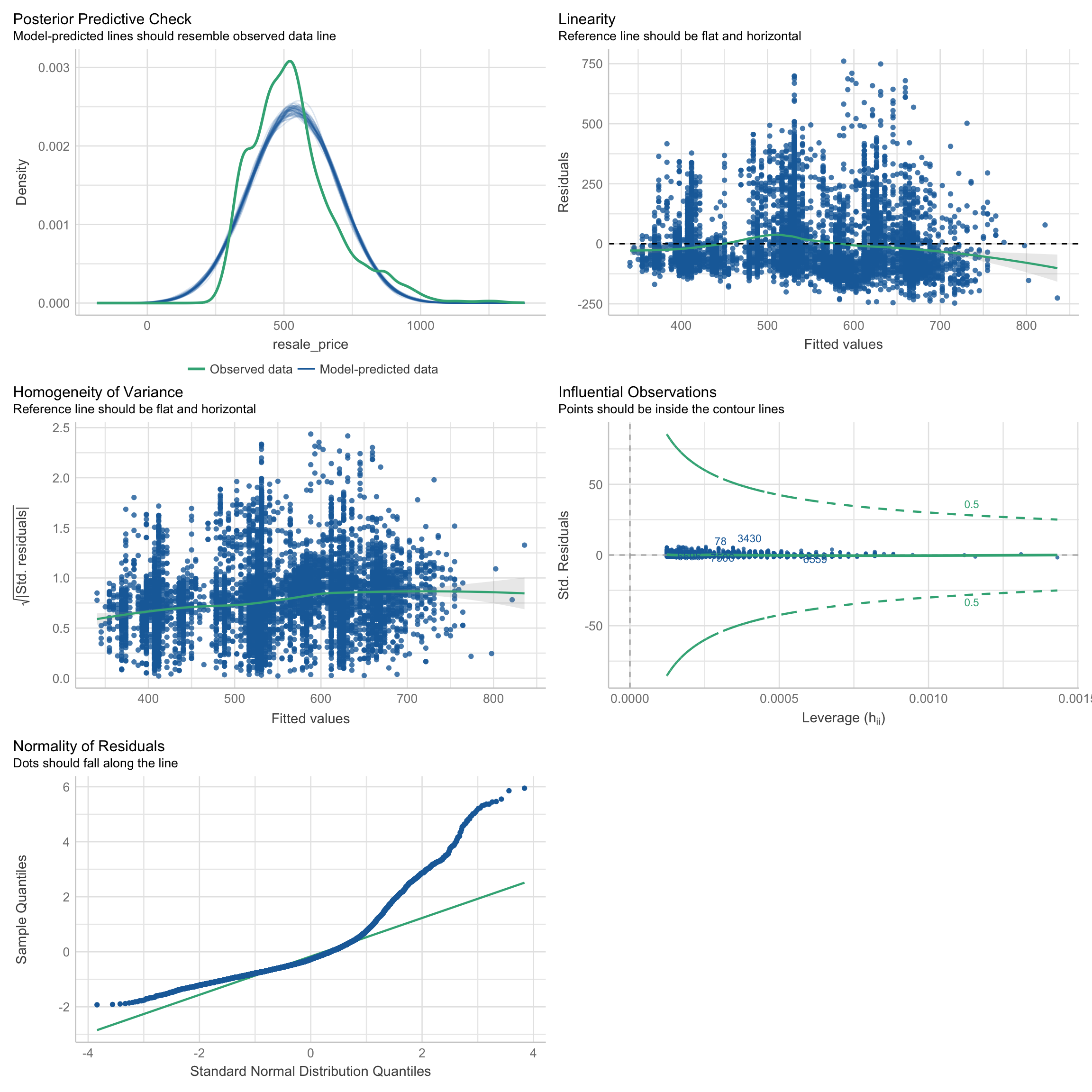
model_lease <- lm(resale_price ~ remaining_lease, data = re)check_model(model_lease)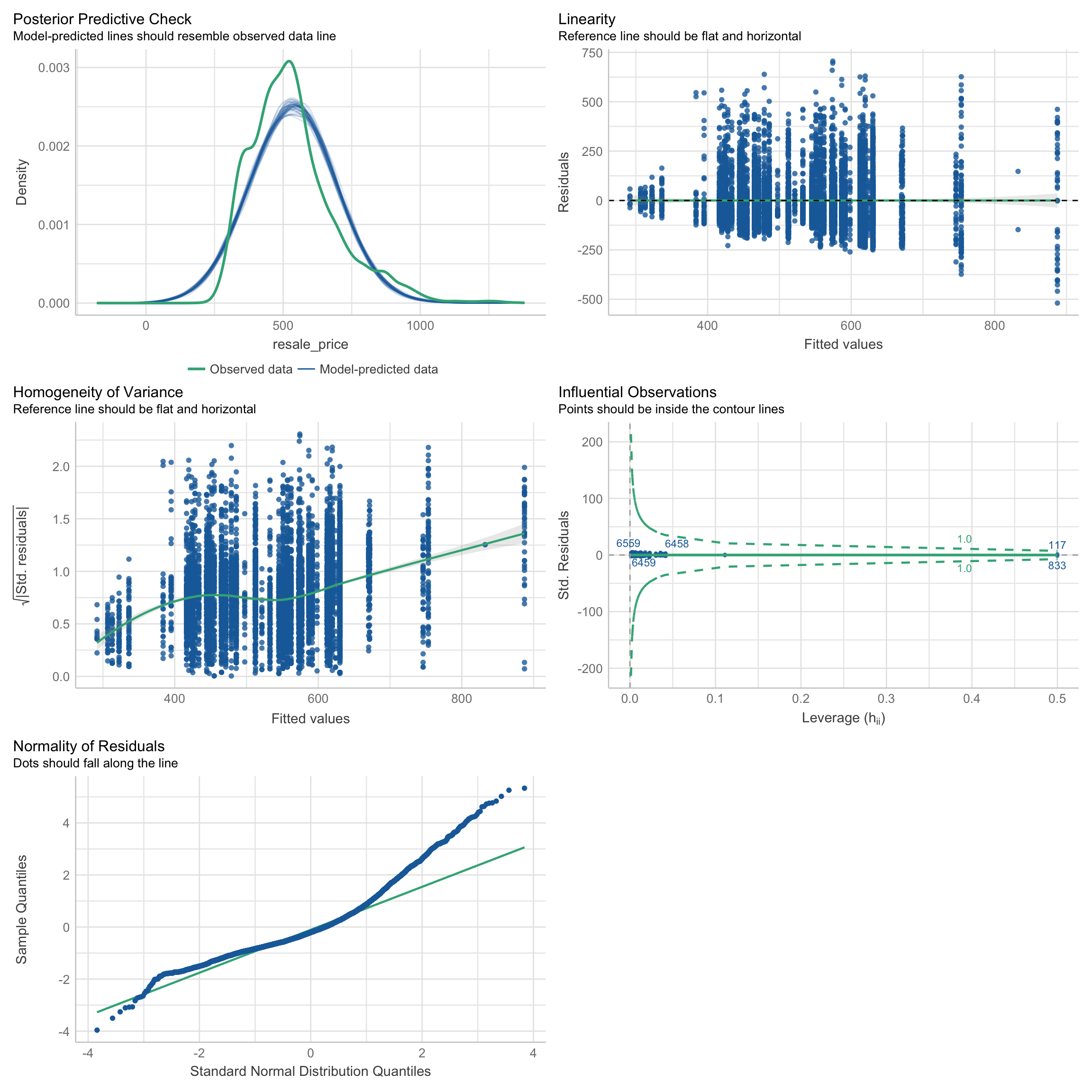
3.2 Visualize Features
3.2.1 Price and Storey of Different Flat Types
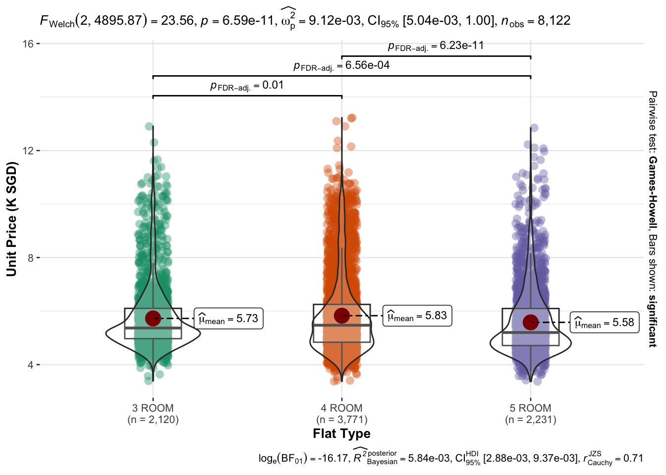
The following static graphs show the price and story range of different flat types, namely 3 ROOM, 4 ROOM, and 5 ROOM. From the plot created by ggbetweenstats( ) and ggbarstats( ), we can tell the mean price and price range and see what the story distribution of each house type is.
The number of 4 ROOM is the highest. The mean price is similar for every flat type. Most of the three-bedroom and five-bedroom unit prices are clustered in the middle and lower reaches and the largest mean price occurs in the 4 room types. As for the story distribution, most resale rooms in the market are located on low floors, which has the largest percentage in 3 ROOM types. This indicates that 3 and 5 room types can be more economic for buyers, and higher stories might have higher prices because of limited second-hand property resources and Singapore’s climate.
ggbetweenstats(
  data = re,
  x = flat_type,
  y = unit_price,
  xlab            = "Flat Type",
  ylab            = "Unit Price (K SGD)",
  type = "p",
  mean.ci = TRUE,
  pairwise.comparisons = TRUE,
  pairwise.display = "s",
  p.adjust.method = "fdr",
  messages = FALSE
) 
ggbarstats(re,
           x = storey_bins,
           y = flat_type)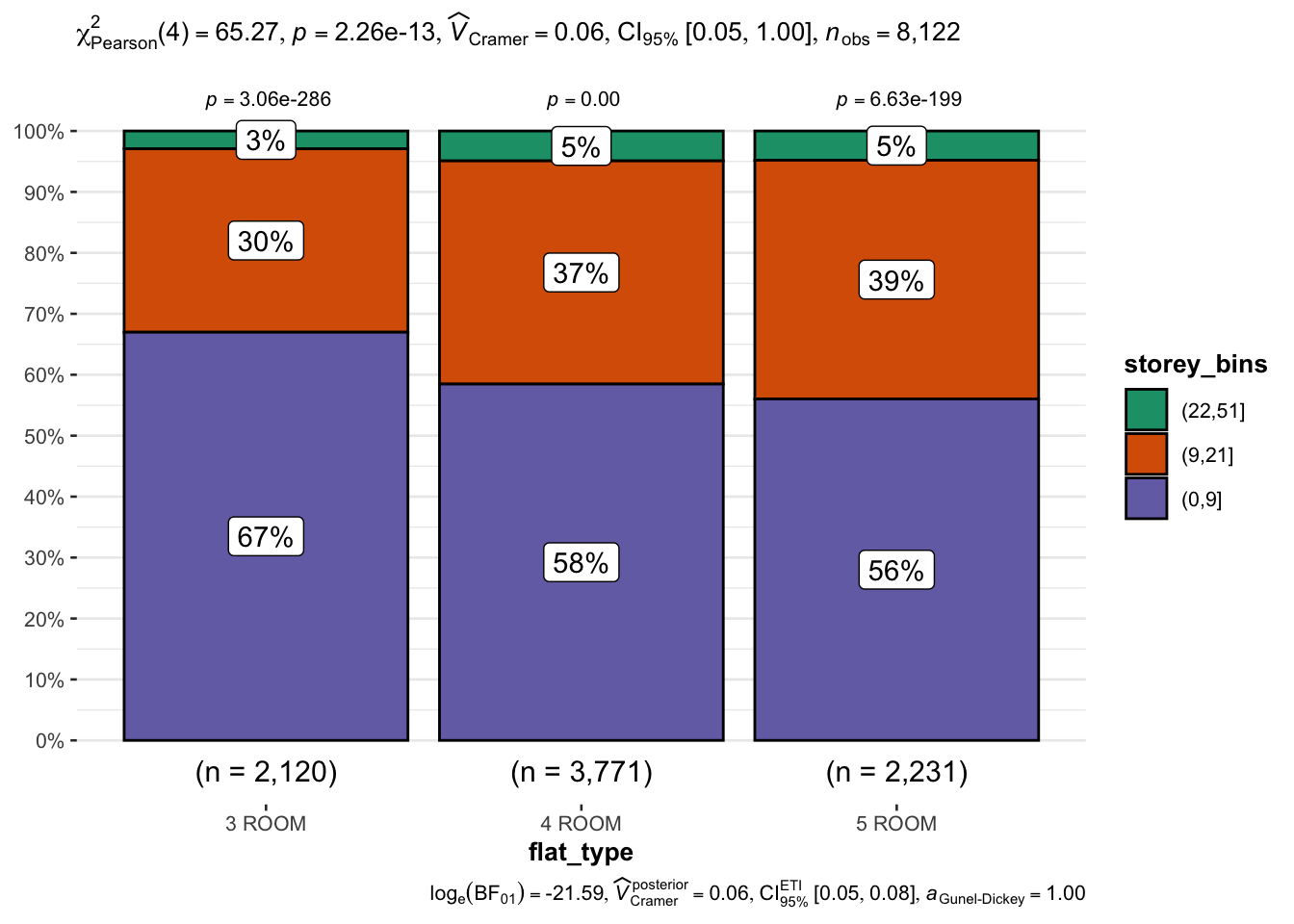
3.2.2 Price by Lease Commence Date and Towns
The dot plot created by plot_ly( ) shows the relationship between the lease commence date and unit price. From the interactive tooltip label on hovering, we can tell the town and flat types the property belong to and have some insights into their relationship.
From the plot, we can see the new flat often sells at higher prices, but there are still many exceptions. For example, some old 3 rooms can have high unit prices because of their location. To specify the influence of locations, the line chart of the price created by giraffe( ) in different towns is shown. Additionally, many rooms at a higher level are much more expensive than their counterparts, which indicates the story can have a tremendous impact on the unit price of resale houses.
plot_ly(data = re,
        x = ~lease_commence_date,
        y = ~unit_price,
        color = ~storey_bins,
        text = ~paste("Town:", town,
                      "<br>Type:", flat_type)) %>%
  layout(title = "Relationship of Lease Commence Date with Unit Price", xaxis = list(title = "Lease Commence Date (year)"), yaxis = list(title = "Unit Price (K SGD)" ), legend = list(title=list(text="<b> Storey Bins </b>")))
avg_price <- aggregate(re$unit_price, by = list(re$town), mean)avg_price$x=round(avg_price$x,2)
head(avg_price) Group.1 x
1 ANG MO KIO 5.92
2 BEDOK 5.44
3 BISHAN 6.67
4 BUKIT BATOK 5.49
5 BUKIT MERAH 7.21
6 BUKIT PANJANG 5.18p_avg_price <- ggplot(data = avg_price, mapping = aes(x = reorder(Group.1, -x), y = x, group = 1)) + geom_line(colour = 'steelblue', size = 2) + geom_point() + xlab('') + ylab("Unit Price (K SGD)") + theme(axis.text.x = element_text(angle = 45, hjust = 1, vjust = 1)) + labs(title = "Unit Price of Different Towns") + theme(plot.title = element_text(size=12,hjust=0.5)) + geom_point_interactive(aes(tooltip = x, data_id = x)) + scale_y_continuous(limits = c(3, 9))
girafe(ggobj = p_avg_price,
width_svg = 6,
height_svg = 6*0.618)3.3 Visualize Correlation
To substantiate the findings in the visualization of the features, a correlogram is used to show key elements related to unit prices. The feature of the lease commence date is omitted in the graph because its P is larger than 0.05.
ggstatsplot::ggcorrmat(data = re, cor.vars = c(6:7,10,13),
ggcorrplot.args = list(outline.color = "black",
                         hc.order = TRUE,
                         tl.cex = 10),
  title    = "Correlogram for resale dataset",
  subtitle = "Four pairs are no significant at p < 0.05"
)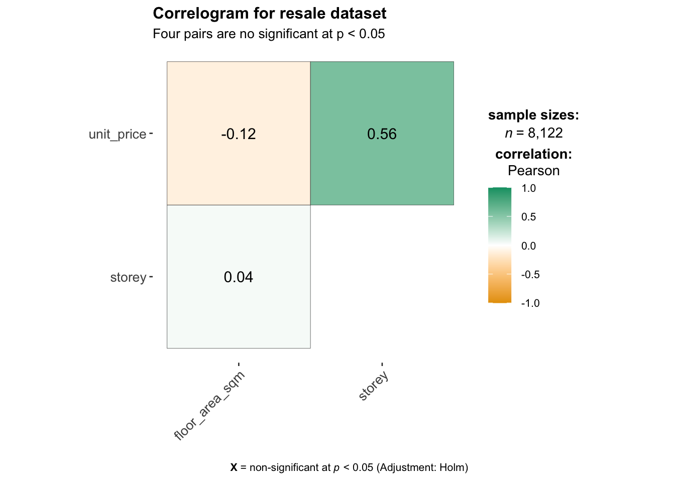
After the correlogram, clustering is adopted to categorize different house types. By using fviz_nbclust( ), it can be seen the best number for clustering is 4. K-means (introduce “floor_area_sqm”, “resale_price”, “unit_price”) is used to do modeling and present the statistics in terms of “town”and “storey_bins”in a table. The summarized features of four types of properties are listed in the table, and a dot plot is created to visualize the clustering of different categorizations by using ggplot2( ).
dim(re)[1] 8122 13fviz_nbclust(re[c("floor_area_sqm","resale_price","unit_price")], kmeans, method = "wss")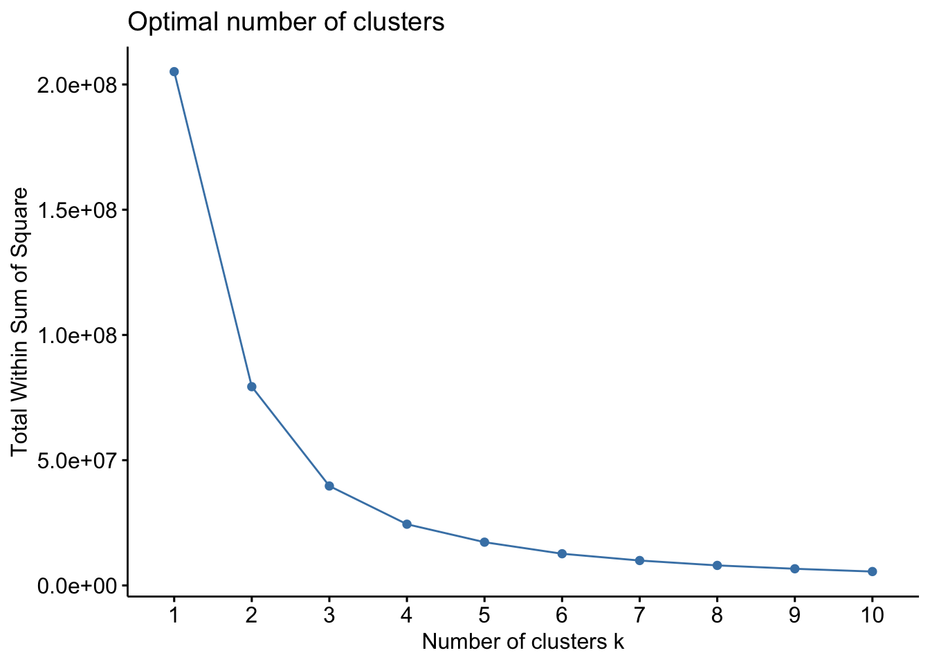
re.kmeans <- kmeans(re[c("floor_area_sqm","resale_price","unit_price")], centers = 4, nstart = 25)
table(re.kmeans$cluster)
   1    2    3    4
3402 647 2437 1636 table(re$town, re.kmeans$cluster)
                    1   2   3   4
  ANG MO KIO       55  48 182  41
  BEDOK           100  13 227  86
  BISHAN           25  41  18  57
  BUKIT BATOK      82  18 114  54
  BUKIT MERAH      40 105  85  78
  BUKIT PANJANG   153   4  71  54
  BUKIT TIMAH       6   6   4   4
  CENTRAL AREA     19  27  15   9
  CHOA CHU KANG   271   0  80  77
  CLEMENTI         35  35  82  43
  GEYLANG          49  23 110  30
  HOUGANG         162  12 125  93
  JURONG EAST      49   0  71  26
  JURONG WEST     247   0 181  51
  KALLANG/WHAMPOA  57  88  83  73
  MARINE PARADE    19  14  24   6
  PASIR RIS       118   1   3  73
  PUNGGOL         395  14  63 173
  QUEENSTOWN       14 101  77  54
  SEMBAWANG       150   0  35  42
  SENGKANG        457  13  74 162
  SERANGOON        45   8  37  32
  TAMPINES        232  18 110 133
  TOA PAYOH        30  58 120  60
  WOODLANDS       339   0 163  49
YISHUN 253 0 283 76table(re$storey_bins, re.kmeans$cluster)
             1    2    3    4
  (0,9]   2080  163 1820  812
  (9,21]  1272  286  609  726
  (21,22]    0    0    0    0
(22,51] 50 198 8 98aggregate(re[c("floor_area_sqm","resale_price","unit_price")], list(re.kmeans$cluster),mean) Group.1 floor_area_sqm resale_price unit_price
1 1 99.79865 517.4858 5.278806
2 2 106.14529 903.6884 8.654521
3 3 74.18182 376.2775 5.140513
4 4 107.06968 667.8437 6.407326| No. | Size | Price | Storage | Location Distribution |
|---|---|---|---|---|
| 1 | Middle | Moderate | Mainly low level and middle level, few high level | Punggol, Woodlands, Choa Chu Kang |
| 2 | Small | Cost-effective | Mainly low level | Yishun, Bedok, Woodlands |
| 3 | Large | Pricey | Mainly high level | Central Area, Bukit Merah, Kallang, Queenstown |
| 4 | Large | Moderate | Mainly low level and middle level, few high level | Bedok, Hougang, Punggol, Sengkang, Tampines |
p_cluster <- ggplot(data = re[c("floor_area_sqm","resale_price","unit_price")], mapping = aes(x = floor_area_sqm, y = unit_price, color = factor(re.kmeans$cluster)))
p_cluster <- p_cluster + geom_point(pch = 20, size = 3)
p_cluster + scale_colour_manual(values = c("skyblue2", "orange", "green3","red"))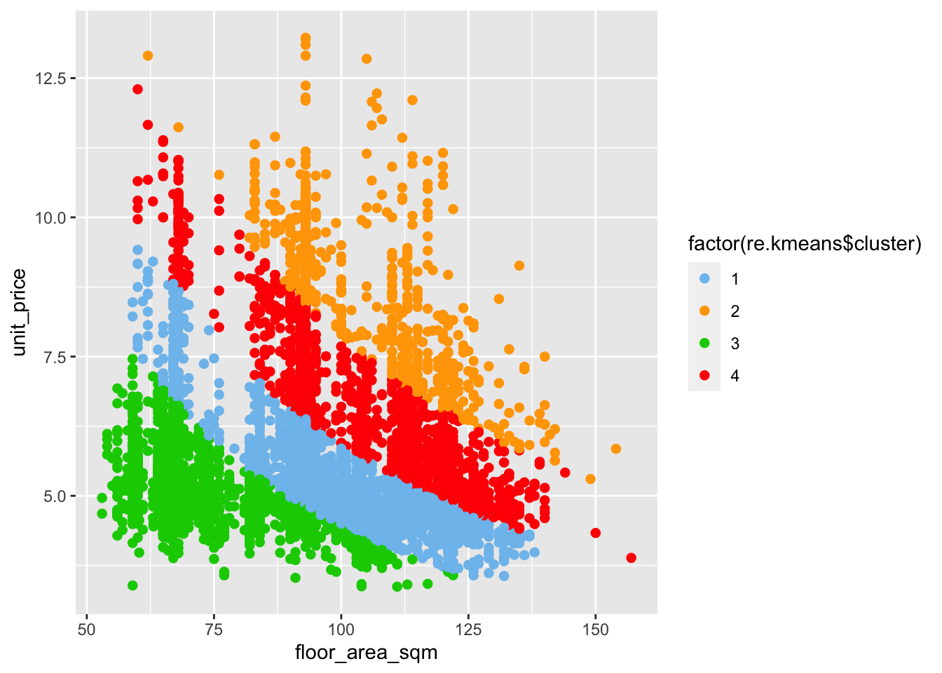
4. Learning Point
In this take-home exercise, interactive and statistic visualization R packages, such as plotly, ggiraph, ggstatsplot are applied to uncover the patterns of resale prices. My key takeaways are:
Rstudio is a powerful tool when doing interactive visualizations, which provides more options for audience to select details for customized viewing. In this assignment, I find it difficult to integrate various information together as there are many elements that should be taken into consideration. Additionally, if a project contains data modeling, a special design must be adopted to make the graph both lively and understandable.
When introducing statistical methods into the visualization analysis, the graph can provide more details. Having a basic understanding of statics is essential for us to do data modeling, and I still need to improve my skills in doing it since I often lack creative ideas in arranging and interpreting data.