In-class Exercise 4

pacman::p_load(plotly, DT, patchwork, ggstatsplot, ggside, readxl, performance, parameters, see, tidyverse)

exam_data <- read_csv("data/Exam_data.csv")

plot_ly(data = exam_data,
        x = ~ENGLISH,
        y = ~MATHS,
        color = ~RACE)

p <- ggplot(data=exam_data, 
            aes(x = MATHS,
                y = ENGLISH)) +
  geom_point(dotsize = 1) +
  coord_cartesian(xlim=c(0,100),
                  ylim=c(0,100))

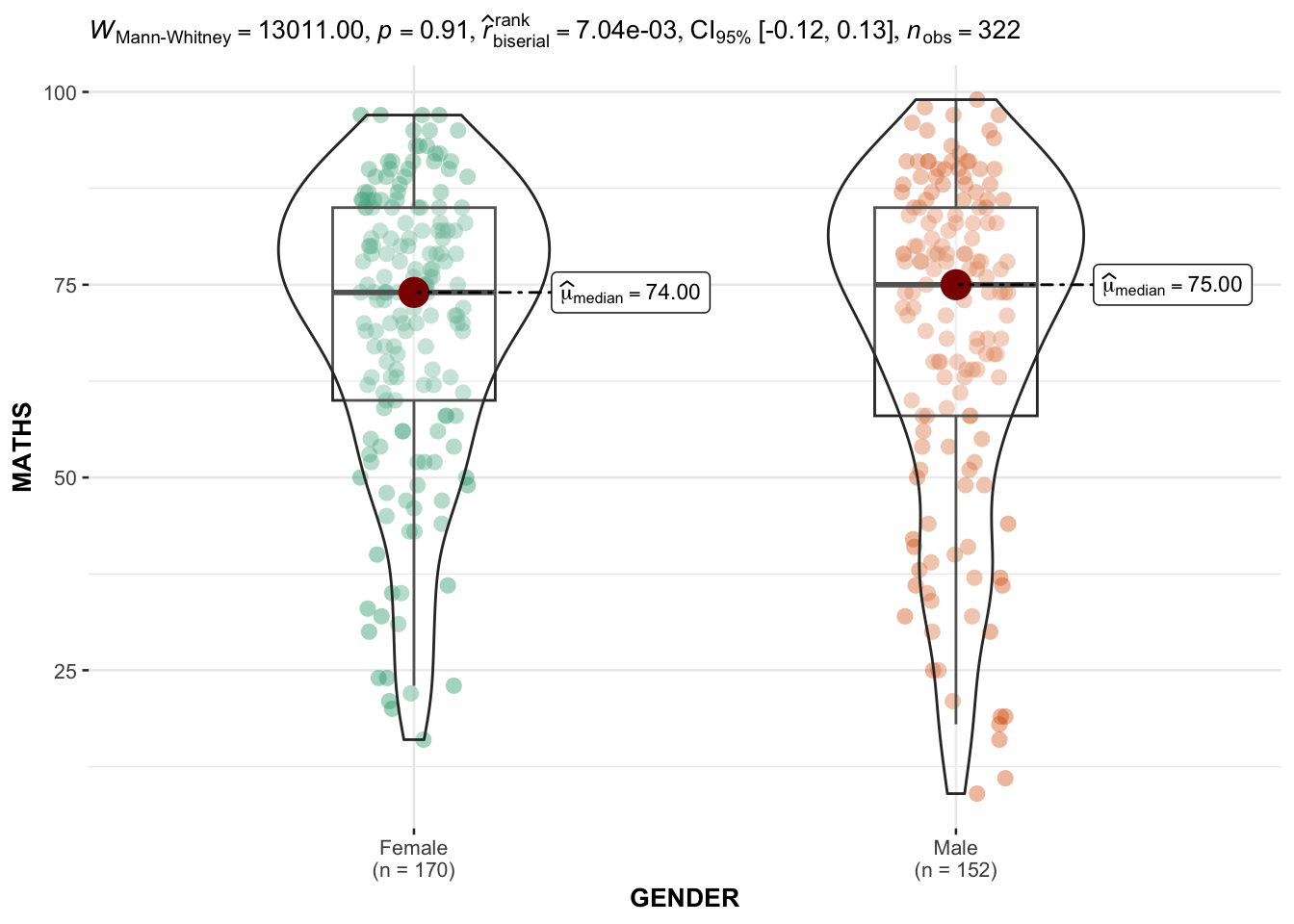
ggplotly(p)

ggbetweenstats(data = exam_data,
  x = GENDER, 
  y = MATHS,
  type = "np",
  messages = FALSE
)

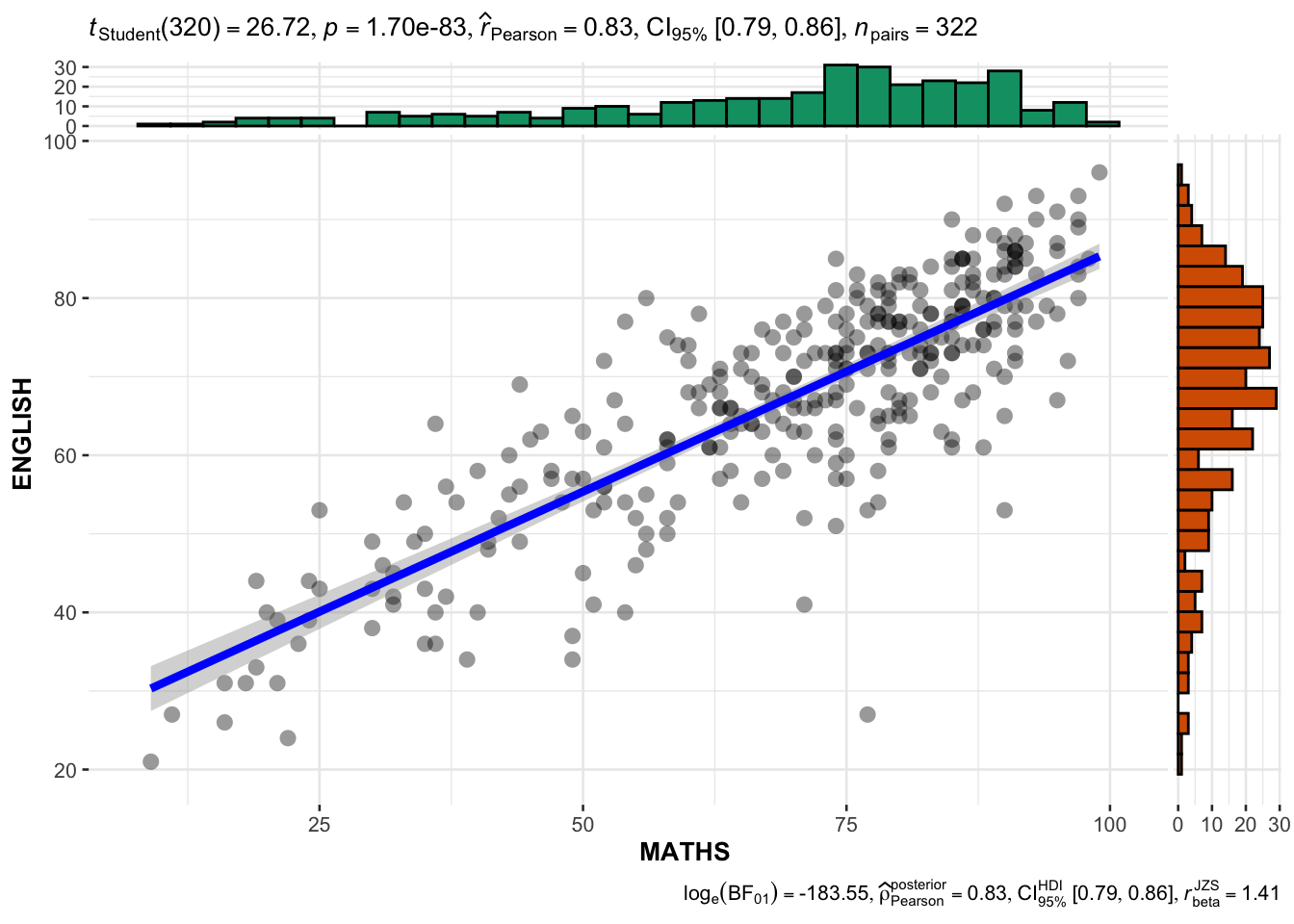
ggscatterstats(
  data = exam_data,
  x = MATHS,
  y = ENGLISH,
  marginal = TRUE,
  )

car_resale <- read_xls("data/ToyotaCorolla.xls", 
                       "data")

model <- lm(Price ~ Age_08_04 + Mfg_Year + KM + 
              Weight + Guarantee_Period, data = car_resale)

check_c <- check_collinearity(model)
plot(check_c)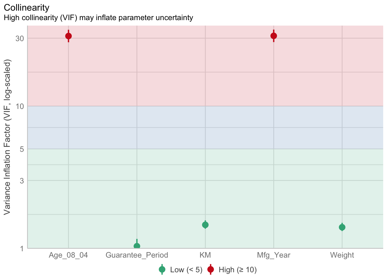

model1 <- lm(Price ~ Age_08_04 + KM + 
              Weight + Guarantee_Period, data = car_resale)

check_n <- check_normality(model1)
plot(check_n)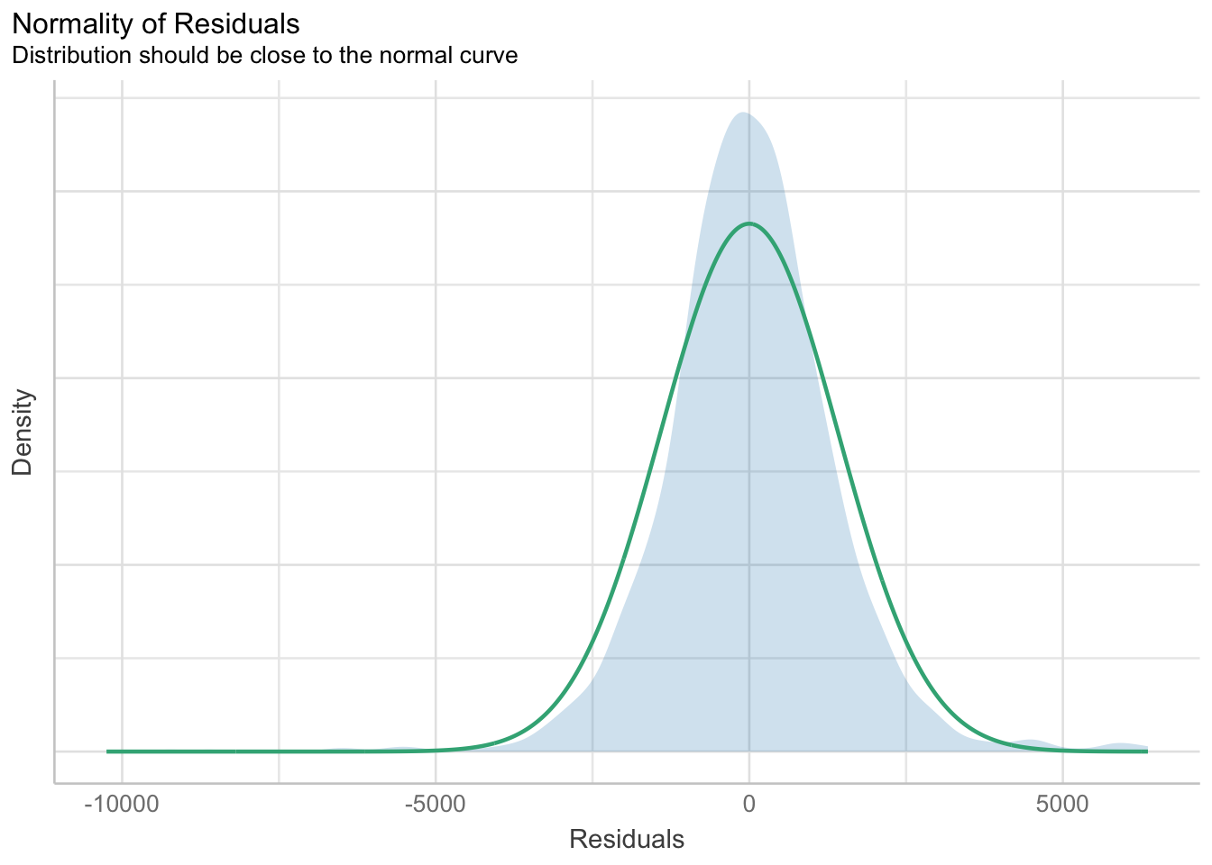

check_h <- check_heteroscedasticity(model1)
plot(check_h)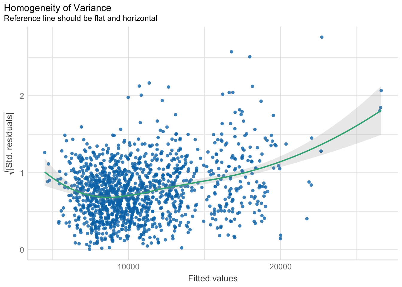

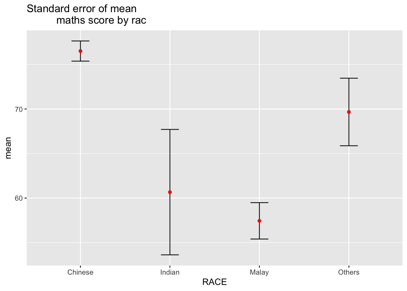
my_sum <- exam_data %>%
  group_by(RACE) %>%
  summarise(
    n=n(),
    mean=mean(MATHS),
    sd=sd(MATHS)
    ) %>%
  mutate(se=sd/sqrt(n-1))
knitr::kable(head(my_sum), format = 'html')

RACE	n	mean	sd	se
Chinese	193	76.50777	15.69040	1.132357
Indian	12	60.66667	23.35237	7.041005
Malay	108	57.44444	21.13478	2.043177
Others	9	69.66667	10.72381	3.791438

ggplot(my_sum) +
  geom_errorbar(
    aes(x=RACE, 
        ymin=mean-se, 
        ymax=mean+se), 
    width=0.2, 
    colour="black", 
    alpha=0.9, 
    size=0.5) +
  geom_point(aes
           (x=RACE, 
            y=mean), 
           stat="identity", 
           color="red",
           size = 1.5,
           alpha=1) +
  ggtitle("Standard error of mean 
          maths score by rac")